This post is the first of a series of posts on model parameter tuning: We will see code to tune Random Forest models with a technique called grid search. Random Forests is a popular ensemble learning method, introduced in its “current” form by Leo Breiman in a same-titled paper. Random forests can be used for classification or regression and offer “protection” from the overfitting that is sometimes observed in single decision trees.
Random Forest performance can be tuned, tweaking a number of parameters.
In this example we will tweak the following three parameters: 1. The split criterion used to choose the variable that splits the data in best way in every step of tree construction aka estimator 2. The minimal number of instances that can form a leave of the trees aka Node Weight 3. The number of trees that will form the ensemble
A typical way to find the optimal values of these parameters is grid search, i.e. specifying a set of possible parameter values, computing all models for them and choosing the best combination according to some performance metric. In essence it is a brute force search method.
Our tools & Data
We will be examining the performance of Random Forests as implemented by package CORElearn, on the titanic passenger list dataset as offered in rpart.plot package.
 .
.
We will be using the caret package for performance metrics,purr for its mapping functions & ggplot for plotting.
Modeling
We will be using 70% of the data to train the models and the rest 30%, using caret:: createDataPartition that automaticaly handles class balance in the split sets. We will be trying trying to predict if a passenger survived according to passenger class, her age,sex, number of siblings/spouses and number of parents/children aboard the ship.
We will be using three spliting criteria chosen from the 37 offered by CORElearn for classification purposes: 1. Gini Index 2. AUC distance between splits. 3. Information Gain Our minimum leaf membership will be tested from 1 to 5 and we’ll be creating ensembles for 10 to 110 trees with a step of 25, as a toy example.
grid_search_vars <- list(minNodeWeightRF = seq(1,5,2),
                         rfNoTrees = seq(10,110,25),estimators= c("Gini","DistAUC", "InfGain")) %>%  purrr::cross_df()

kable(grid_search_vars[1:5,], caption = "First 5 rows of parameter matrix",format = 'markdown') | minNodeWeightRF | rfNoTrees | estimators |
|---|---|---|
| 1 | 10 | Gini |
| 3 | 10 | Gini |
| 5 | 10 | Gini |
| 1 | 35 | Gini |
| 3 | 35 | Gini |
#Function that accepts the parameters and computes model
fit_mod<-function(x,y,z){

  fit.rand.forest = CoreModel(survived~., data=train_set, model="rf", selectionEstimator=z, minNodeWeightRF=x, rfNoTrees=y)

  return(fit.rand.forest)
}

#Map values to function: When testing a lot of values this can take a while
res<-pmap(list(grid_search_vars$minNodeWeightRF,grid_search_vars$rfNoTrees,grid_search_vars$estimators),fit_mod)


#Predict for test set and calculate performance metrics
preds<- lapply(res, function(x) predict(x, newdata=test_set, type="class") ) %>%
lapply(., function(x) as.data.frame(t(c(confusionMatrix(x,test_set$survived)$overall,                               confusionMatrix(x,test_set$survived)$byClass))))%>%bind_rows()
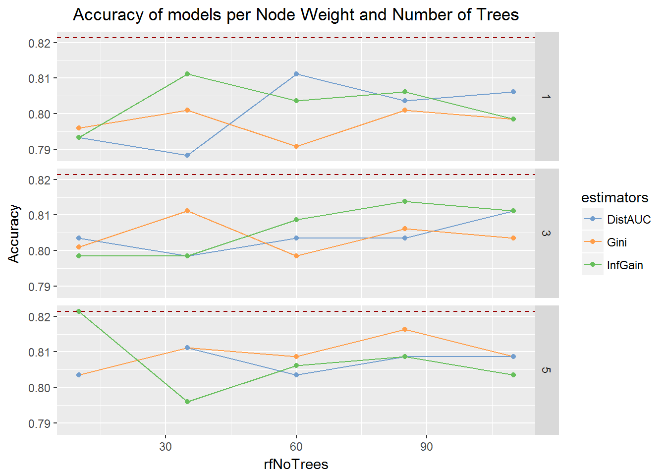
Best results in terms of Accuracy (82.14%) are produced by an ensemble of 10 trees with a minimum of 5 members per leaf.
df<-bind_cols(grid_search_vars,preds)%>% arrange(desc(Accuracy), rfNoTrees, minNodeWeightRF)

kable(df[1:7,1:10] , caption = "Top 10 results - along with Accuracy Metrics",format = 'markdown') | minNodeWeightRF | rfNoTrees | estimators | Accuracy | Kappa | AccuracyLower | AccuracyUpper | AccuracyNull | AccuracyPValue | McnemarPValue |
|---|---|---|---|---|---|---|---|---|---|
| 5 | 10 | InfGain | 0.8214286 | 0.6122103 | 0.7798538 | 0.8580676 | 0.6173469 | 0 | 0.0231510 |
| 5 | 85 | Gini | 0.8163265 | 0.6031942 | 0.7743770 | 0.8534209 | 0.6173469 | 0 | 0.0770999 |
| 3 | 85 | InfGain | 0.8137755 | 0.5992381 | 0.7716426 | 0.8510934 | 0.6173469 | 0 | 0.1601719 |
| 1 | 35 | InfGain | 0.8112245 | 0.5963487 | 0.7689110 | 0.8487631 | 0.6173469 | 0 | 0.4157977 |
| 3 | 35 | Gini | 0.8112245 | 0.5963487 | 0.7689110 | 0.8487631 | 0.6173469 | 0 | 0.4157977 |
| 5 | 35 | Gini | 0.8112245 | 0.5879077 | 0.7689110 | 0.8487631 | 0.6173469 | 0 | 0.0075020 |
| 5 | 35 | DistAUC | 0.8112245 | 0.5911141 | 0.7689110 | 0.8487631 | 0.6173469 | 0 | 0.0481310 |
We can plot the results for a better overview of performance.
ggplot(df,aes(x=rfNoTrees,y=Accuracy,colour=estimators))+
  geom_line()+geom_point()+ geom_hline(aes(yintercept=max(df$Accuracy)), colour="#990000", linetype="dashed")+
  facet_grid(minNodeWeightRF ~ .)+labs(title="Accuracy of models per Node Weight and Number of Trees")+
  scale_colour_tableau('tableau10medium')+theme(plot.title = element_text(hjust = 0.5))
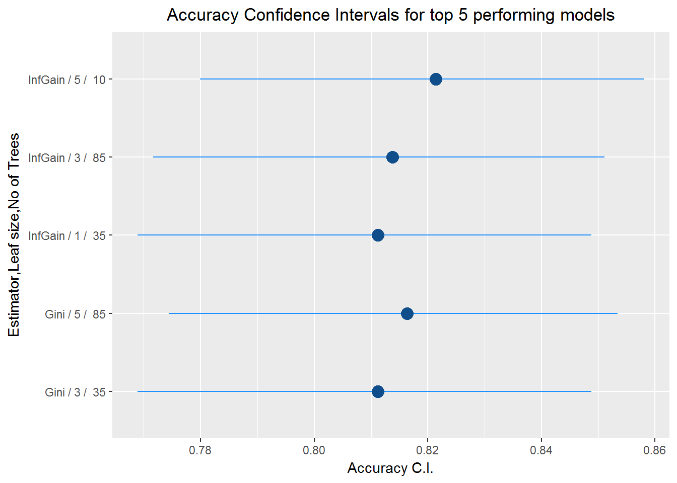
df_top5<-df[1:5,]
df_top5$id<-paste(df_top5$estimators,"/",df_top5$minNodeWeightRF,"/ ",df_top5$rfNoTrees)

ggplot(df_top5,aes(x=Accuracy,y=id))+
  geom_segment(aes(x=AccuracyLower, y=id,xend=AccuracyUpper,yend=id),data=df_top5,colour="dodgerblue1")+
  geom_point(shape=16,colour="dodgerblue4",size=4)+
  labs(x="Accuracy C.I." , y="Estimator,Leaf size,No of Trees", title = "Accuracy Confidence Intervals for top 5 performing models")+
  theme(plot.title = element_text(hjust = 0.5))